
Machine Learning with Splunk: Testing Logistic Regression vs Support Vector Machines (SVM) using the ML Toolkit
By: Brent McKinney | Splunk Consultant
If you’ve ever spent time working with Machine Learning, it’s highly likely you’ve come across Logistic Regression and Support Vector Machines (SVMs). These 2 algorithms are amongst the most popular models for binary classification. They both share the same basic goal: Given a sample x, how can we predict a variable of interest y?
For example, let’s say we have a dataset with samples (x) containing the following,
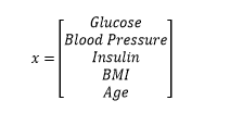
and we want to determine a single variable y: Is this person diabetic or not?
Logistic Regression and SVMs are perfect candidates for this!
The problem now lies in finding the means to test this on a sizeable dataset, where we have hundreds or thousands of samples. Coding machine learning algorithms can become quite a task, even for experienced developers. This is where Splunk comes in!
Splunk’s Machine Learning Toolkit makes testing ML algorithms a breeze. The Machine Learning Toolkit is an app, completely free to download on Splunkbase and allows users to visualize and compare results from ML algorithms quickly, without having to code them.
To stay consistent with our previous example, I will be demonstrating this with a public dataset from Kaggle.com, in the form of a CSV file. This dataset includes real data, that is already labeled and clean. Since our data is properly labeled, this can be will serve as a supervised learning problem. This simply means that our task will learn a function that maps an input (our x features) to an output (our y value – diabetic or not) based on the labeled items. I’ve posted the link to the MLTK app, as well as the dataset used in this example, as sources at the bottom of this page.
To install the MLTK app: Once you’ve downloaded the Machine Learning Toolkit from Splunkbase, log into your Splunk instance, and click the Apps dropdown at the top of the screen. Select “Manage Apps” and then click the button “Install app from file”. From here select Choose File and select the MLTK app folder (no need to untar the file, Splunk will unpack the folder on the server!). Click Upload.
To upload a csv file: You can upload the csv file by clicking Settings>Lookups>Lookup table files>New Lookup Table File. Select MLTK for the app, our csv as the upload file, and give a name with the .csv extension (diabetes.csv). Then go to Settings>Lookups>Lookup definition>New Lookup Definition to define the lookup. We’ll select the MLTK app, “diabetes” for the name, “File-based” for the type, and the csv file for the Lookup file.
Once the Machine Learning Toolkit has been installed, and the dataset file has been uploaded to Splunk, we can get to work.
From your Splunk instance, navigate to the Machine Learning Toolkit app by selecting it from the “App” dropdown menu at the top of the screen.
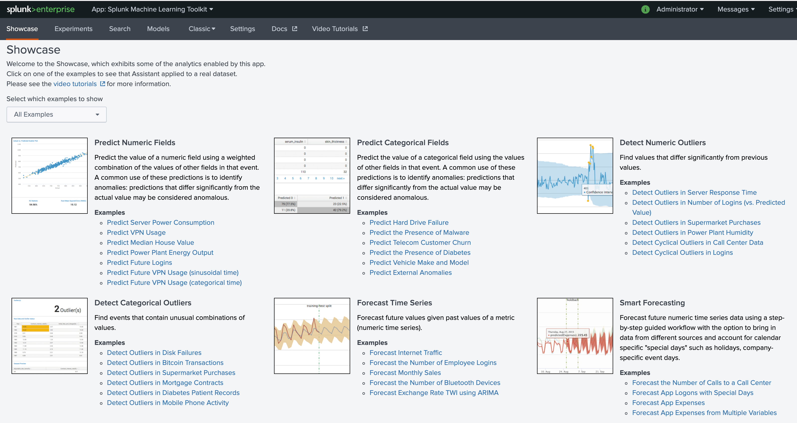
From here we can see there are several options available, each depending on the problem you are trying to solve. We want to categorize our data into 2 categories: diabetic and not diabetic. So for our example, we will use “Predict Categorical Fields”.
To start, select “Experiments” from the navigation bar, and then “Create New Experiment”. Select the appropriate experiment type, then add a title and description.
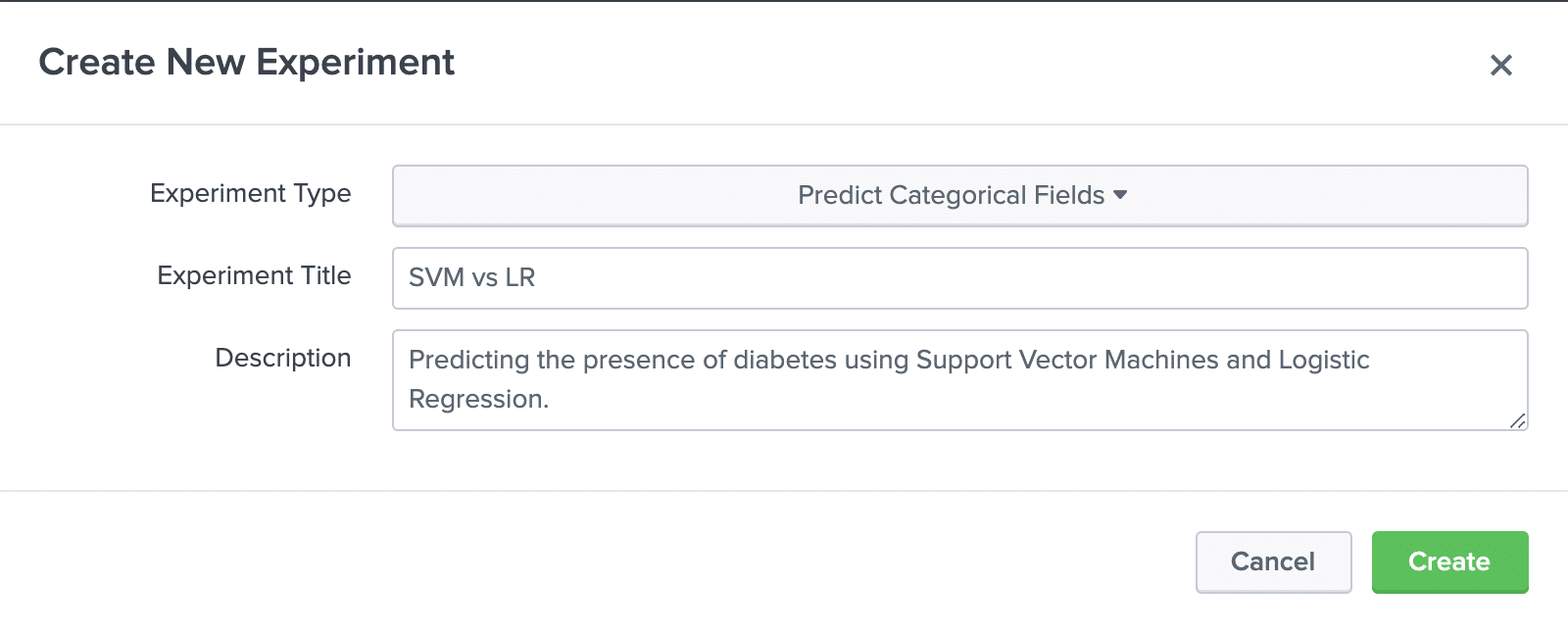
Once all looks good, select Create.
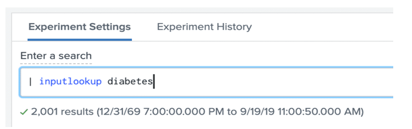
Now we are brought to the experiment screen. To use our diabetes dataset, we will need to use the SPL inputlookup command in the search bar. Note the search must begin with a | as this is a generating command.
This will return the data we uploaded from the CSV file.
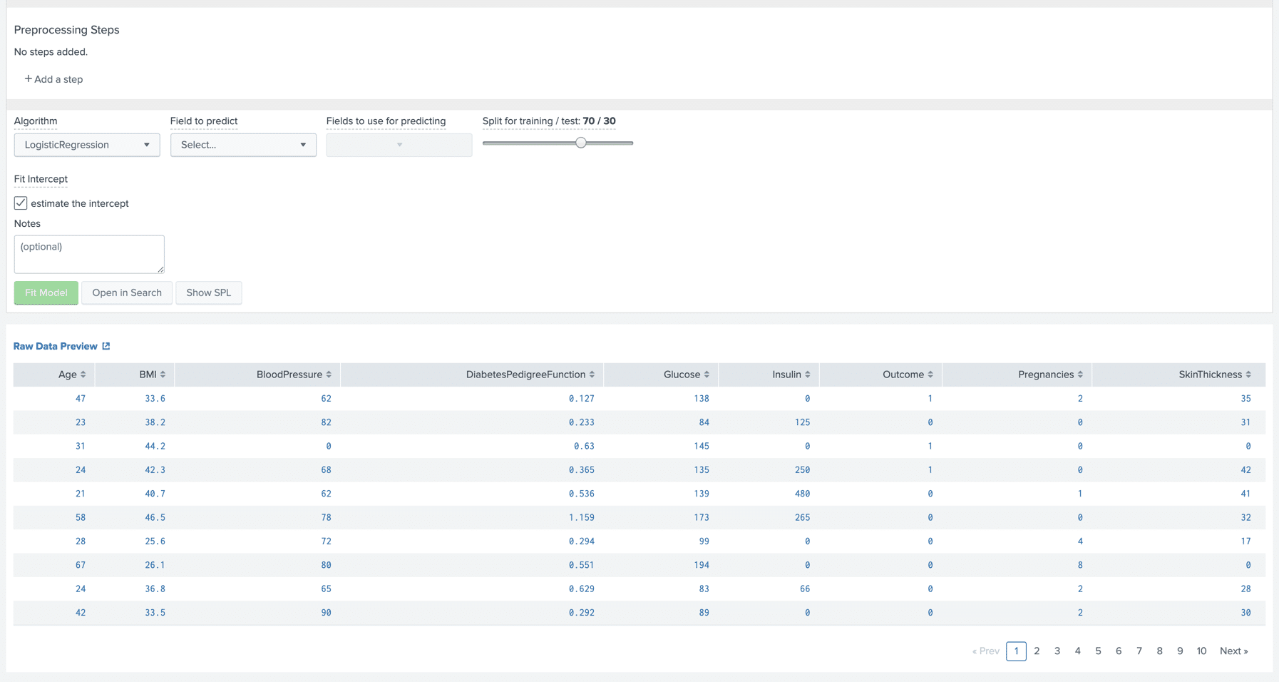
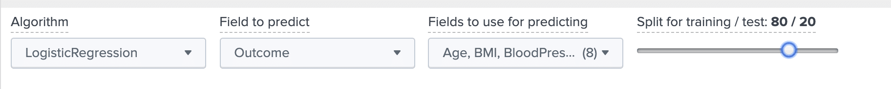
As we can see, there are a few parameters that need to be set. The first being the algorithm we want to use. We will be testing Logistic Regression and SVM. The default is Logistic Regression so we can leave it as-is for now.
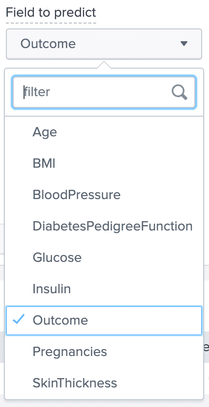
The next parameter is “Field to Predict”. This represents the variable we want to discover, y. This list is populated with fields found in our csv file. In our example, our y variable is “Outcome”, which gives a value of 1 for samples that are diabetic, and a value of 0 for samples that are NOT diabetic.
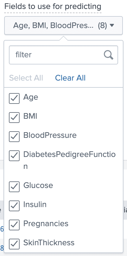
The next parameter is “Fields to use for predicting”. As the name implies, these are the variables that make up our feature sample x. The algorithms will use these features to determine our Outcome variable. The more relevant fields we select here, the more accurate our algorithms will be when calculating a result, so in this case we will select all of them.
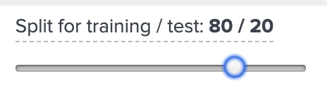
Once these parameters have been set, all we need to do is decide how we want to split the data into training and testing.
Machine Learning algorithms use the training data to determine a function that most accurately produces the desired output. So to achieve the best accuracy, we want to use a majority of the data for training. Once the algorithm is trained on the dataset, it runs this function on the test data and gives an output based on the samples it saw during training. For this example, I will use 80% for training, and 20% for testing.
(Note, while we want to use as much training data as possible, we must have some test data. If we use 100% of the data for training, then any test data will have already been seen by the algorithm, and therefore not give us any insightful results.)
Now that all of our parameters are set, we are ready to see results!
Select Fit Model to run Logisitic Regression on our data.
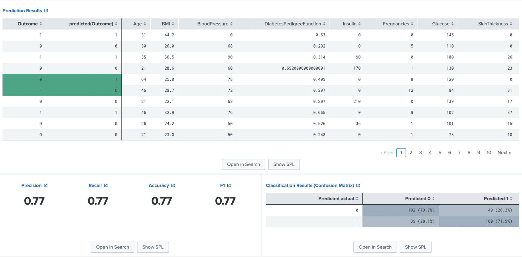
Once the algorithm is finished, we are given 3 panels.
The first returns a results table containing our test data. The columns on the right of the bold line show our original x features for each sample. The columns on the left of the bold line show the output that the algorithm predicted for each sample, compared to the actual output in the dataset, for each sample, highlighting the ones it got wrong.
The panel on the bottom left shows the degree of accuracy of the algorithm for our given dataset. From this we can conclude that if we were to give this model a new sample, it would determine whether or not the sample is diabetic or not with a 77% degree of accuracy.
The bottom right panel gives a little more detail, showing how well the algorithm did at predicting each outcome. We can see that for our particular example, it did slightly better at determining samples that were not diabetic, as opposed to samples that were.
Now let us compare this to a SVM model. Considering that we want to use the same dataset and parameters, all we need to do is change the algorithm.

Once that is set, we can select Fit Model to run SVM on our data.
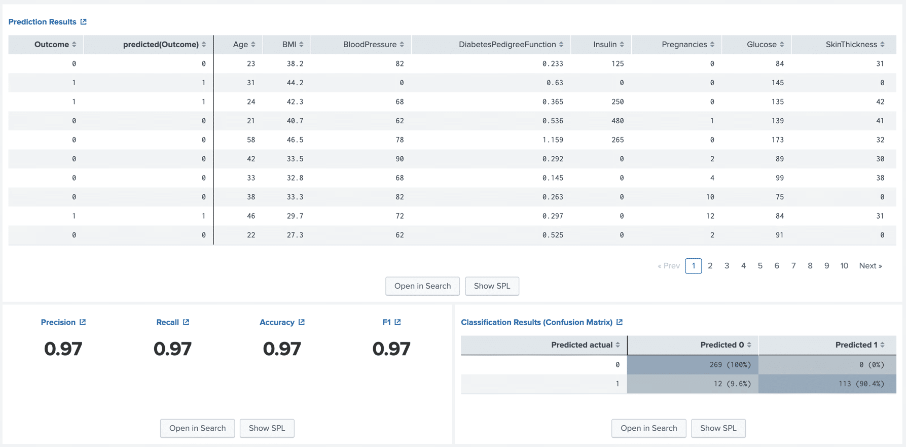
Right away we can see that using Support Vector Machines gives us substantially better results than Logisitic regression. Both algorithms give the same details format, but we can see that using SVM resulted in a 97% accuracy when predicting on our test data, in comparison to LR resulting in 77%.
To conclude, Splunk’s Machine Learning Toolkit provides an easy-to-use environment for testing and comparing Machine Learning algorithms. In this demonstration, we used Splunk and Machine Learning to create models to predict whether a given sample is diabetic or not. While this demonstration focused on SVMs and Logistic Regression, there are many more algorithms available in Splunk’s Machine Learning Toolkit to play around with, including Linear Regression, Random Forests, K-means Clustering, and more!
Link to download Machine Learning Toolkit app:
https://splunkbase.splunk.com/app/2890
Link to download dataset used in this example:
https://kaggle.com/johndasilva/diabetes
Want to learn more about Machine Learning with Splunk? Contact us today!