
Slice And Dice: Comparing Values Over Specific Times
Part One: Day Over Week
Marvin Martinez | Splunk Consultant
If you’re lost, you can look and you will find it: Time OVER time. Sometimes, data can’t just be visualized sequentially. Often, it is most useful to compare data across specific points in time. In this 4-part series, I will be outlining some interesting ways to help visualize data points across specific points in time, namely day over week (i.e. this past Thursday versus the last three Thursdays) and hour over week (this past Thursday at 1 p.m. to last three Thursdays at 1 p.m.). The first installment will focus on the day-over-week visualization that allows the user to quickly visualize the last four Thursdays (or any other day of the week) overlayed on top of each other to quickly determine any discrepancies between them.
For example, let’s say you’re monitoring sales throughout the day. You notice that sales seemed to spike up at 8 p.m. yesterday, but you’re curious if it is spiking up at that same hour every Thursday or if the peaks are happening at different times and how big those discrepancies are.
Splunk has some very handy, albeit underrated, commands that can greatly assist with these types of analyses and visualizations. Additionally, it can be difficult to clearly display the appropriate context and intent of the visualizations, so it is imperative to clearly delineate what the data points represent on the charts themselves. We’ll explore both situations in this article, including some sample SPL to help you get where you need to get with your own data.
To achieve this, we’ll use the timewrap command, along with the xyseries/untable commands, to help set up the proper labeling for our charts for ease of interpretation.
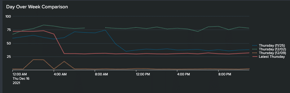
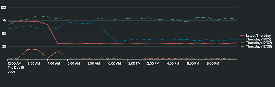
In the end, our Day Over Week Comparison chart will look like this. The chart shows each Thursday across the past four weeks, overlayed on top of each other. (Note that you could go back as far as your data lets you go. This is just how far back we went for the purpose of this article.)
This is the search that was used for the panel shown above. Each of our events has a TotalSales field that we are using as our value to chart.
| index=”test” ….
| eval Date = strftime(_time,”%m/%d”), Day = strftime(_time,”%A”), Hour=strftime(_time,”%H”)
| fields _time, “TotalSales”, Hour, Day, Date
| where Day=”Thursday”
| timechart span=1h count(TotalSales) as TotalSales
| timewrap 1w series=short
| rename TotalSales _s0 as LatestDay, TotalSales _s1 as WeeksBack1, TotalSales _s2 as WeeksBack2, TotalSales _s3 as WeeksBack3, TotalSales _s4 as WeeksBack4
| untable _time FieldName FieldValue
| eventstats latest(_time) as LatestDate
| eval WeekNum = substr(FieldName,-1)
| eval FieldName = CASE(FieldName = “LatestDay”, “Latest Thursday”,1=1,”Thursday (” . strftime(relative_time(LatestDate,”-” . WeekNum . “w@h”),”%m/%d”) . “)”)
| xyseries _time FieldName FieldValue
| table _time “Thursday*” “Latest *”
Let’s break this search down and explain what is going on here. The first four lines are setting up our data. We create fields to store the specific Date, Day, and Hour for our values as well as filter out only the information for the specific day we are looking to compare.
The timewrap command requires a timechart command before it, so execute a timechart command to get the data the way you need it (in this case, spanned across an hour). Note that you are already only looking at a specific day across multiple weeks.
Now execute the timewrap command, spanning one-week intervals and using the series=short option. This creates the resulting fields as “TotalSales_s0…” and so on. This is helpful since they can then be easily renamed in the next command to make it easier to understand which date each series represents. At this point, if you ran the search just up to the rename command after the timewrap, your visualized result should look something like this:
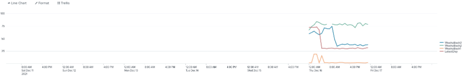
This is almost there, but still not intuitive when viewing. Let’s work on that!
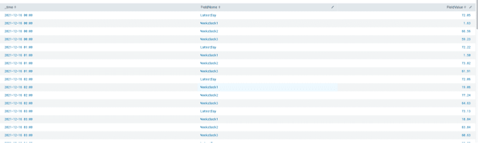
The “| untable _time FieldName FieldValue” command will reformat the data as shown below, with a FieldName and FieldValue column, containing the field names and values, respectively. We can use this to rename our fields to make them easier to understand.
The following eventstats and eval commands do just that. Eventstats will determine what the latest date is in the remaining events. We will use this to help determine the actual date of the other line values. The eval commands grab the last number from the FieldName and then use a CASE statement to update the name of the field. If the FieldName is “LatestDay,” then we know it is the most recent day in our data set. Otherwise, we will update the field name to be the name of the day followed by a relative_time offset going back the WeekNum number of weeks.
| eval WeekNum = substr(FieldName,-1)
| eventstats latest(_time) as LatestDate
| eval FieldName = CASE(FieldName = “LatestDay”, “Latest Thursday”,1=1,”Thursday (” . strftime(relative_time(LatestDate,”-” . WeekNum . “w@h”),”%m/%d”) . “)”)
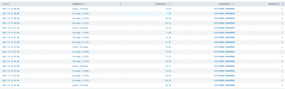
After these commands, your results should look something like this. Note that the FieldName is now intuitively named.
From here, all we need to do is use the xyseries command to turn these field names back into columns for our chart.
| xyseries _time FieldName FieldValue
At this point, the chart will look pretty much the way we need it to.
However, we need this to be as easy to read as possible! Looking at the legend, the fields aren’t quite in the right order. Note how “Latest Thursday” is at the top but the other series do not follow sequentially in the right time order. We can fix that with the table command to control the ordering of our chart. Order the table command with _time, followed by the “Thursday” entries (use the * to denote a wildcard) and, finally, the “Latest *” field at the very end.
| table _time “Thursday*” “Latest *”
Now, your chart looks like this. Much better! The dates in the legend now show in ascending order and are easier to follow.
 Figure 1: Dotted lines were added via dashboard panel options for fieldDashStyles and lineDashStyle
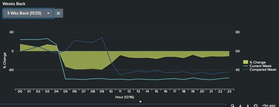
In the next installment, we will create a panel that will allow us to compare one specific day from a prior week to the latest day and visualize the percentage changes between the two throughout every hour of that day. A sneak peek is shown below. Until next time!
Visualizing data doesn’t have to be complicated. Check out Part Two of our Slice and Dice Series and stay tuned for Part Three coming Spring 2023.
Contact one of our exceptional Splunk Consultants today so we can put your data to work for you!